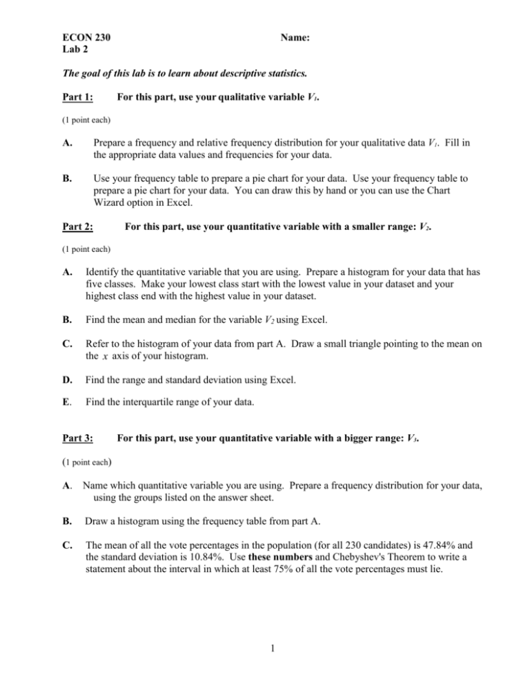
ECON 230
Lab 2
Name:
The goal of this lab is to learn about descriptive statistics.
Part 1:
For this part, use your qualitative variable V1.
(1 point each)
A.
Prepare a frequency and relative frequency distribution for your qualitative data V1. Fill in
the appropriate data values and frequencies for your data.
B.
Use your frequency table to prepare a pie chart for your data. Use your frequency table to
prepare a pie chart for your data. You can draw this by hand or you can use the Chart
Wizard option in Excel.
Part 2:
For this part, use your quantitative variable with a smaller range: V2.
(1 point each)
A.
Identify the quantitative variable that you are using. Prepare a histogram for your data that has
five classes. Make your lowest class start with the lowest value in your dataset and your
highest class end with the highest value in your dataset.
B.
Find the mean and median for the variable V2 using Excel.
C.
Refer to the histogram of your data from part A. Draw a small triangle pointing to the mean on
the x axis of your histogram.
D.
Find the range and standard deviation using Excel.
E.
Find the interquartile range of your data.
Part 3:
For this part, use your quantitative variable with a bigger range: V3.
(1 point each)
A.
Name which quantitative variable you are using. Prepare a frequency distribution for your data,
using the groups listed on the answer sheet.
B.
Draw a histogram using the frequency table from part A.
C.
The mean of all the vote percentages in the population (for all 230 candidates) is 47.84% and
the standard deviation is 10.84%. Use these numbers and Chebyshev's Theorem to write a
statement about the interval in which at least 75% of all the vote percentages must lie.
1
ECON 230
Lab 2
Name:
Excel Directions

To make a pie chart using a frequency table, first type the first two columns of your frequency
table into Excel:
First, highlight the two columns that have your categories and the frequencies. Then select the Chart
Wizard.
Step 1: Select chart type “Pie” and click “Next.”
Step 2: You should be able to click “Next” and there should be a preview of the pie chart
Step 3: Give your chart a title. Then click on the “Data Labels” tab. Select the category name
and percentage options. Click “Next.”
Step 4: Click “Finish.”

For your quantitative data in Part 2, you may find your statistics using Excel.
To use Excel to do statistics, we first need to add the Analysis ToolPak.
For Excel 2003: To do this, go to Tools on the pulldown menu and choose Add-Ins. Select the
Analysis ToolPak and click OK.
Now select the 40 observations for the variable V2 that you want to summarize. Go to Tools on the
pulldown menu and choose Data Analysis. Then select “Descriptive Statistics” and check the box
that says “Summary statistics.” The summary statistics will be reported in a new worksheet. These
statistics will include the mean and the standard deviation.
For Excel 2007 or later: Click on the button in the upper left and select Excel Options in the box on
the lower right. Then click on “Add-Ins” on the panel on the left. Select the Analysis ToolPak and
then click “Go.”
Click on the Data tab and select “Data Analysis” under the Analysis group. Then select “Descriptive
Statistics” and check the box that says “Summary statistics.” Highlight the observations you want to
find the mean for by putting the cursor in the input range box and selecting the data. The summary
statistics will be reported in a new worksheet. These statistics will include the mean and the
standard deviation.
2
ECON 230
Lab 2
Name:
Particularly on a Mac, there are sometimes problems with Analysis ToolPak. If you have trouble
with the ToolPak, you can find everything you need to find using commands that you type into
Excel. Start by clicking into an empty cell. Then:
1) To find the mean, type “=AVERAGE( ” and then select all the cells that you want to take the
mean of. Finally type “)” and hit enter.
2) To find the median, type “=MEDIAN( ” and then select all the cells that you want to take the
mean of. Finally type “)” and hit enter.
3) To find the standard deviation, type “=STDEV( ” and then select all the cells that you want to
take the mean of. Finally type “)” and hit enter.
4) To find the minimum, type “=MIN( ” and then select all the cells that you want to take the
mean of. Finally type “)” and hit enter.
5) To find the maximum, type “=MAX ( ” and then select all the cells that you want to take the
mean of. Finally type “)” and hit enter.
6) To find the third quartile, type “=PERCENTILE( ” and then select all the cells that you want
to take the mean of. Finally type “,0.75)” and hit enter. This finds the 75th percentile. If you
want to find the first quartile, you should just modify this command as necessary.
3
ECON 230
Lab 2
Name:
Along with your previous lab in your folder, you should hand in just the answer sheets for this
lab.
Answer sheet for elections data:
Part 1:
A)
Party
Frequency
Percentage
Democrat
Republican
Other
B) Pie chart:
Part 2:
A) Quantitative variable: ______________
Histogram:
4
Cumulative
percentage
ECON 230
Lab 2
Name:
B) Mean = _____________
Median = _____________
C) Put the triangle on the histogram you drew in part A)
D) Range = _____________
Standard deviation = _____________
E) Interquartile range = _____________
Part 3:
A) Quantitative variable = _______________
Vote percentage
Frequency
Percentage
Cumulative
percentage
15.01%-29.00%
29.01%-43.00%
43.01%-57.00%
57.01%-71.00%
71.01%-85.00%
B) Histogram:
C) Based on Chebyshev’s Theorem, 75% of all the vote percentages must lie between
$____________________ and $_____________________.
5