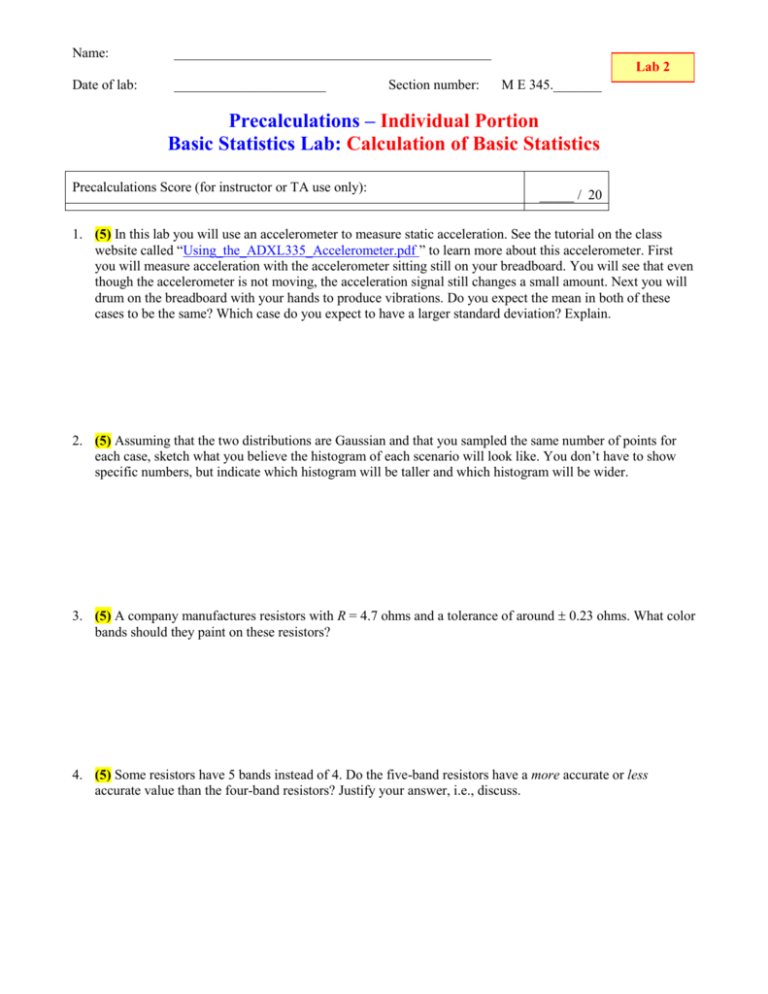
Name:
______________________________________________
Date of lab:
______________________
Lab 2
Section number:
M E 345._______
Precalculations – Individual Portion
Basic Statistics Lab: Calculation of Basic Statistics
Precalculations Score (for instructor or TA use only):
_____ / 20
1. (5) In this lab you will use an accelerometer to measure static acceleration. See the tutorial on the class
website called “Using_the_ADXL335_Accelerometer.pdf ” to learn more about this accelerometer. First
you will measure acceleration with the accelerometer sitting still on your breadboard. You will see that even
though the accelerometer is not moving, the acceleration signal still changes a small amount. Next you will
drum on the breadboard with your hands to produce vibrations. Do you expect the mean in both of these
cases to be the same? Which case do you expect to have a larger standard deviation? Explain.
2. (5) Assuming that the two distributions are Gaussian and that you sampled the same number of points for
each case, sketch what you believe the histogram of each scenario will look like. You don’t have to show
specific numbers, but indicate which histogram will be taller and which histogram will be wider.
3. (5) A company manufactures resistors with R = 4.7 ohms and a tolerance of around  0.23 ohms. What color
bands should they paint on these resistors?
4. (5) Some resistors have 5 bands instead of 4. Do the five-band resistors have a more accurate or less
accurate value than the four-band resistors? Justify your answer, i.e., discuss.
Lab 2, Basic Statistics Lab Page 1
Cover Page for
Lab 2
Lab Report – Group Portion
Introductory Lab: Basic Operation of Common Laboratory Instruments
Name 1:
___________________________________________________
Section M E 345._______
Name 2:
___________________________________________________
Section M E 345._______
Name 3:
___________________________________________________
Section M E 345._______
[Name 4:
___________________________________________________
Section M E 345._______ ]
Date when the lab was performed:
______________________
Group Lab Report Score (For instructor or TA use only):
Lab experiment and results, plots, tables, etc.
_____ / 55
Discussion
_____ / 25
TOTAL
______ / 80
Lab Participation Grade and Deductions – The instructor or TA reserves the right to deduct points for any of
the following, either for all group members or for individual students:







Arriving late to lab or leaving before your lab group is finished.
Not participating in the work of your lab group (freeloading).
Causing distractions, arguing, or not paying attention during lab.
Not following the rules about formatting plots and tables.
Grammatical errors in your lab report.
Sloppy or illegible writing or plots (lack of neatness) in your lab report.
Other (at the discretion of the instructor or TA).
Name
Reason for deduction
Comments (for instructor or TA use only):
Points deducted
Total grade (out of 80)
Lab 2, Basic Statistics Lab Page 2
Basic Statistics Lab: Calculation of Basic Statistics
Author: John M. Cimbala; also edited by Savas Yavuzkurt and Michael Robinson, Penn State University
Latest revision: 12 September 2014
Introduction and Background (Note: To save paper, you do not need to print this section for your lab report.)
The engineering profession is dependent on both accurate and precise representation of experimental data.
Unfortunately, due to inherent uncertainties involved in making measurements, the exact value is often not
obtainable. Consider, for example, measurement of the thickness of a piece of metal. Metal can be purchased in
standard “stock” sizes, such as ¼-inch steel stock  a sheet of steel, nominally 0.2500… inches thick. However,
if the thickness of a specimen is measured carefully at several locations with a precise instrument, such as a
micrometer, you will find that the actual thickness is not perfectly uniform, and is not exactly ¼-inch thick, due
to the manufacturing process. Similarly, many sensors will produce varying results even if the sensor is
measuring a constant value. In this lab you will observe variations in an accelerometer signal. The science of
statistics enables us to quantify such variations, and the associated errors, by introducing parameters such as
mean, standard deviation, etc. Definitions of these parameters are provided in the lecture material.
In this lab, basic statistical analysis, sometimes called multiple point uncertainty analysis will be performed on
samples measured in the lab.
Objectives
1. Become familiar with experimental measurements of thickness and resistance.
2. Learn how to use the Vernier scale on a micrometer
3. Develop an appreciation for errors and uncertainties in experimental measurements.
4. Practice applying statistical techniques to quantify these errors and uncertainties.
5. Practice creating and interpreting histograms and probability density functions.
6. Determine whether a larger sample size produces better statistics.
Equipment
 aluminum metal stock –nominally ½  1 in, cut to 8 inches length (a different piece for each lab group,
but all of them were cut from the same original piece of stock metal)
 Vernier Caliper: sliding type with dual units (inches and cm
 Micrometer: ratchet type with Vernier scale
 digital multimeter (DMM), with appropriate cables as needed
 two cell phones (not supplied; use your own personal cell phones)
 stopwatch (or use the stopwatch app on a third cellphone)
 ADXL335 analog accelerometer
 USB data acquisition system
Lab 2, Basic Statistics Lab Page 3
Procedure
Accelerometer measurements
1. (4) Using the USB data acquisition system in the lab, collect 100 data points from a stationary
accelerometer on your lab bench. Use the MATLAB code “USB1608G_Sample.m ” from the class
website. There is also a tutorial on the class website called “Using_the_ADXL335_Accelerometer.pdf ”
to help you get started. You can decide at what rate to sample the data. Report the statistics of your
sample shown below.
Sample mean = ___________ V
Sample median = ___________ V
Sample mode = ___________ V
Sample standard deviation = ___________ V
2. (2) Write the voltage measured from the accelerometer in standard engineering form, assuming 95%
confidence.
V = ___________ +/- __________ V
3. (4) Use MATLAB to plot a histogram for the data you collected. Include an image of that figure in your
report. Hint: The MATLAB command hist() plots a histogram of a set of data, so hist(chan0) would plot
a histogram of the voltages from channel 0 on the DAQ. Search in the MATLAB help files to find more
information about the hist() command if you want to learn more.
Histogram of stationary accelerometer signal: see attached, Figure number ___________
4. (4) Repeat the experiment above, but this time drum on the lab bench near your breadboard with your
hands to create additional vibrations which you will also measure with the accelerometer. Report the
statistics of your sample shown below.
Sample mean = ___________ V
Sample median = ___________ V
Sample mode = ___________ V
Sample standard deviation = ___________ V
5.
(3) Use MATLAB to plot a histogram for the data you collected.
Histogram of accelerometer signal with additional vibration: see attached, Figure number ___________
Thickness measurements
Note: Each lab station has one Vernier caliper and one micrometer used for accurate measurement of length.
Practice with both. All of them have a Vernier scale, and a resolution of 0.001 in. (e.g., 0.265 inches) when
using the Vernier scale. Some of them also have a digital “odometer” type readout – ignore that part, and use the
Vernier scale instead.
Do not over-tighten the micrometers – they are fragile, and easily broken! Use the outside ratchet to tighten.
1. (2) Measure and record the nominal thickness of the piece of stock metal (in inches). In other words,
round off to the nearest 1/8 inch. (e.g., 1/8, 1/4, 3/8, 1/2 ... inches, which are the standard stock sizes).
Nominal thickness, t = ___________ in
2. Using the Vernier scale on the micrometer for highest precision, measure and record (into Excel) the
thickness (inches) at various positions on the stock metal. Take 30 or more thickness measurements, and
Lab 2, Basic Statistics Lab Page 4
each member should be given a chance to take measurements – a minimum of 10 per person. [One of the
goals of this portion of the lab is to give each student some experience with using the micrometers.] Ask
for assistance in reading the Vernier scale if you are unfamiliar with Vernier scales.
3. If your micrometer has a zero error (non-zero reading when fully closed without the stock metal),
subtract this bias error from each data point before proceeding.
4. Add your names, section number, and computer name (e.g., “Measurement 02”) to the spreadsheet.
Give a copy of the Excel file to the TA via jump drive or e-mail. [Later on, we will combine your data
with those of other lab groups so that you can analyze a larger sample – the population.]
5. (5) Create a nice-looking histogram from your thickness data. Use Sturgis’ rule and/or the Rice rule as
guides for how many bins to use. The actual number of bins depends on your choice of bin values.
Specify your own bin values, as discussed in learning module “Histograms.pdf ”, so that the histogram
is nice-looking and neat.
Note: The Histogram macro can be found under the Data tab in the Data Analysis menu. It should be
located on the far right of the Data tab under Analysis.
If Data Analysis is not located under the Data tab follow the directions below:
1. Click on the File for EXCEL 2xxx in the top left corner of the Excel screen and then click on the
Excel Options from the dropdown menu
2. From the Excel Options window, select Add-ins from the menu on the left, then click on Go.
3. Check the box next to Analysis ToolPak and click Ok.
4. Click Yes to any windows that may pop up.
Histogram of sample thickness data, our lab group only: see attached, Figure number ___________
Statistical analysis of the entire population of thickness data (all samples from all lab groups in your section)
1. Your instructor/TA will gather the thickness data from all the lab groups in your section, and he/she
will collect all the data from in your section into one Excel file so that you can perform statistical
analysis on the whole population (we call this the population, although it is really just a larger sample).
Get this Excel file from your instructor or TA. If the file is not ready yet, move to the cell phone part.
2. (5) Create a nice-looking histogram from the thickness data. Use Sturgis’ rule and/or the Rice rule as
guides for how many bins to use. The actual number of bins depends on your choice of bin values.
Specify your own bin values, as discussed in learning module “Histograms.pdf ”. (You can also ask help
from TA), so that the histogram is nice-looking and neat.
Histogram of population thickness data (all lab groups): see attached, Figure number ___________
3. (5) Convert your histogram into a probability density function (PDF) Hint: Divide each value (number
of samples in each bin) by n, the total number of measurements, and divide also by the bin width to
generate f(x). Plot f(x) versus xmid, the mid value of each x, with appropriate scales and labels on the
axes. Caution: Excel’s histogram plots are based on the maximum x value for each bin. However, for
proper conversion to normalized form, the middle value of x in each bin must be used instead.
PDF of population thickness data [f(x) vs. x]: see attached, Figure number ___________
4. Convert your PDF into a standard normalized PDF, i.e., f(z) vs. z instead of f(x) vs. x. Be careful to
properly convert both x and f(x) using the transformations z   x    /  and f ( z )    f ( x) , as
discussed in learning module “Probability_density_functions.pdf ”. Plot f(z) vs. z on a scatter plot,
using symbols only.
5. (5) On the same plot, plot the standard Gaussian distribution function (using a curve only) for
comparison. The Gaussian distribution can be created in Excel using its definition or the function
1
exp   z 2 / 2  = NORMDIST(z,0,1,FALSE).
“NORMDIST”. Namely, for a given z, f  z  
2
PDF of thickness data [f(z) vs. z] compared to Gaussian PDF: see attached, Figure number ___________
6.
(7) Record all the following data for the “population” of thickness data:
Lab 2, Basic Statistics Lab Page 5
Population mean = ___________ in
Population median = ___________ in
Population mode = ___________ in
Population standard deviation = ___________ in
Thickness in engineering format = ___________ +/- __________ in
Population mean – nominal value = ___________ in
Some fun with cell phones
1. In this section, we will take several measurements of how long it takes for a cell phone call to go
through. Get two cell phones – one will be the caller and one will be the receiver.
2. Call the receiver phone from the caller phone. With a stopwatch, time how long it takes from the time
you hit the SEND button until the first ring on the receiver phone. Record the time (seconds) as
precisely as possible (typically to 1/100 of a second) in an Excel spreadsheet.
3. Repeat as many times as you want – no fewer than 20. Again, the more data you take the better should
be your statistics.
4. (4) Calculate the sample mean, sample median, sample mode (if it exists), and sample standard
deviation.
Sample mean = ___________ s
Sample median = ___________ s
Sample mode = ___________ s
Sample standard deviation = ___________ s
5. (5) Draw a nice-looking histogram of the data.
Histogram of cell phone data: see attached, Figure number ___________
Lab 2, Basic Statistics Lab Page 6
Discussion Questions
1. (5) Statisticians often use standard deviation divided by mean ( S / x ) as a nondimensional measure of
the overall precision of a sample. Calculate S / x for your lab group’s stationary acceleration
measurements and cell phone samples on a percent basis. Which set of measurements is more precise?
Justify your answer and discuss.
2. (5) List some of the reasons that one cell phone call may take longer to go through than another cell
phone call, even when calling from the same phone to the same phone.
3. (5) Did the histograms you produced for each of the accelerometer trials match your expectations?
Explain.
4. (5) Look at the histogram for your lab group’s cell phone measurements. Does the distribution appear to
be nearly Gaussian? If not, what aspect(s) of the histogram lead you to your conclusion? Discuss.
5. (5) Finally, compare and discuss the histograms of the thickness measurements for your group’s data
only versus those of your entire lab section (which we are calling the population). Does a larger sample
yield better statistics and better agreement with a standard bell curve shape? Should it? Discuss.