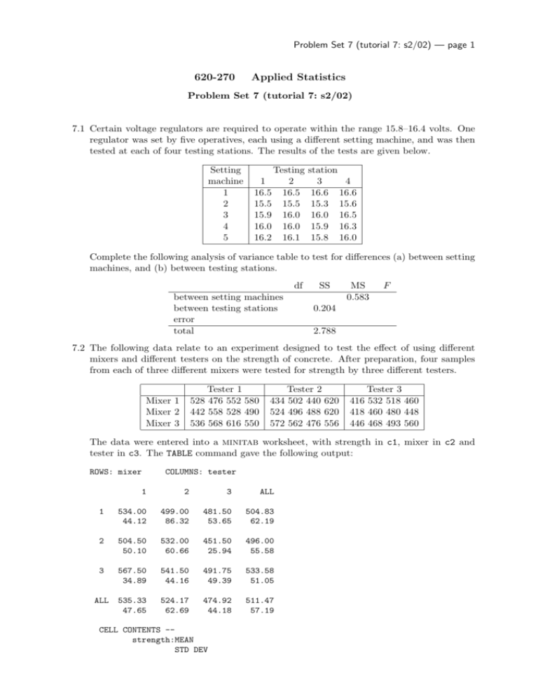
Problem Set 7 (tutorial 7: s2/02) — page 1
620-270
Applied Statistics
Problem Set 7 (tutorial 7: s2/02)
7.1 Certain voltage regulators are required to operate within the range 15.8–16.4 volts. One
regulator was set by five operatives, each using a different setting machine, and was then
tested at each of four testing stations. The results of the tests are given below.
Setting
machine
1
2
3
4
5
1
16.5
15.5
15.9
16.0
16.2
Testing
2
16.5
15.5
16.0
16.0
16.1
station
3
4
16.6 16.6
15.3 15.6
16.0 16.5
15.9 16.3
15.8 16.0
Complete the following analysis of variance table to test for differences (a) between setting
machines, and (b) between testing stations.
df
between setting machines
between testing stations
error
total
SS
MS
0.583
F
0.204
2.788
7.2 The following data relate to an experiment designed to test the effect of using different
mixers and different testers on the strength of concrete. After preparation, four samples
from each of three different mixers were tested for strength by three different testers.
Tester 1
528 476 552 580
442 558 528 490
536 568 616 550
Mixer 1
Mixer 2
Mixer 3
Tester 2
434 502 440 620
524 496 488 620
572 562 476 556
Tester 3
416 532 518 460
418 460 480 448
446 468 493 560
The data were entered into a minitab worksheet, with strength in c1, mixer in c2 and
tester in c3. The TABLE command gave the following output:
ROWS: mixer
COLUMNS: tester
1
2
3
ALL
1
534.00
44.12
499.00
86.32
481.50
53.65
504.83
62.19
2
504.50
50.10
532.00
60.66
451.50
25.94
496.00
55.58
3
567.50
34.89
541.50
44.16
491.75
49.39
533.58
51.05
ALL
535.33
47.65
524.17
62.69
474.92
44.18
511.47
57.19
CELL CONTENTS -strength:MEAN
STD DEV
Problem Set 7 (tutorial 7: s2/02) — page 2
(a) Plot (by hand) the nine means in an “interaction plot”, (like the plots on page 70
of the notes). Do you think there are (i) differences between mixers? (ii) differences
between testers? (iii) an interaction between mixers and testers?
(b) We will firstly fit an additive model to the data.
i. Use the information in the above minitab output to compute the total SS, SS
due to mixer and SS due to tester.
ii. Construct the ANOVA table for an additive model.
iii. Test whether there is any difference between the mixers.
iv. Test whether there is any difference between the testers.
v. Find an estimate of σ.
(c) We now wish to fit an interactive model to the data.
i. The SS due to interaction is 6161. Construct an ANOVA table for the interactive
model.
ii. Test whether an additive model is appropriate.
7.3 The following data are percentage yields in a chemical process.
temperature level 1
temperature level 2
Catalyst 1
91 93
90 94
Catalyst 2
88 86
95 94
Catalyst 3
93 92
90 87
The following output is from minitab:
SOURCE
temp
catalyst
INTERACTION
ERROR
TOTAL
DF
1
2
2
6
11
SS
4.08
5.17
68.17
17.50
94.92
MS
4.08
2.58
34.08
2.92
(a) Test whether the interaction is significant. Explain the interaction using four of the
six means for the different treatment combinations.
(b) Use a suitable model to test whether the main effects are significant. Comment on
whether this is a useful thing to do.
7.4 An experiment was conducted to compare the yields of orange juice for six different juice
extractors. Because of a possibility of a variation in the amount of juice per orange from
one batch to another, equal weights of oranges from each batch were randomly assigned
to each extractor. This process was repeated for fifteen batches. The amount of juice was
recorded for the oranges sent to each extractor from each batch, resulting in the following
incomplete analysis of variance table:
df
between batches
between extractors
error
total
SS
159.29
84.71
MS
F
338.33
(a) What type of experimental design was used? What were the experimental units?
What were the treatments?
(b) Complete the ANOVA table.
(c) Do the data provide sufficient evidence to indicate a difference in the mean amount
of juice extracted by the six extractors? Explain.
Problem Set 7 (tutorial 7: s2/02) — page 3
7.5 When metal pipe is buried in soil it is desirable to apply a coating to retard corrosion.
Four coatings are under consideration for use with pipe that will ultimately be buried in
three types of soil. An experiment to investigate the effects of these coatings and soils was
carried out by first selecting 12 pipe segments and applying each coating to three segments.
The segments were then buried in soil for a specified period in such a way that each soil
type received one piece with each coating. The resulting data (depth of corrosion) is given
below.
Coating
1
2
3
4
Soil type
1
2
3
68 53 54
53 51 48
44 42 47
51 43 52
(a) Assuming that there is no interaction between coating and soil type, test for possible
effects of coating and soil type.
(b) Find 95% confidence intervals for differences between the mean of level 1 and the
other levels, for any significant factors.
7.6 The following observations are standardised yields from 24 plots divided into four blocks,
each containing six similar plots. Three treatments were applied twice in each block, as
indicated.
block 1
block 2
block 3
block 4
total
control
0, 1
–1, –2
0, 2
3, 5
8
Analysis of Variance for y
source
df
ss
blocks
81
treatments
error
total
144
treatment F
1, –1
2, 1
1, 2
2, 4
12
treatment G
2, 0
1, 2
4, 3
7, 9
28
total
3
3
12
30
48
ms
(a) For these data, show that the sum of squares due to treatments is equal to 28, and
complete the above analysis of variance table.
Assuming an additive model with independent normally distributed errors having equal
variances:
(b) test the significance of the treatment effects.
(c) find an estimate of the error variance.
(d) find a 95% confidence interval for the mean yield with treatment G.
(e) find a 95% confidence interval for the effect of treatment G, i.e., the difference in
mean yield for treatment G compared to the control (no treatment).
(f) Use the following minitab output to find the interaction sum of squares and hence
how significant the interaction is. A large contribution to the interaction is made by
one cell — which one is it?
Problem Set 7 (tutorial 7: s2/02) — page 4
MTB > print c1-c4
Row
y block treat
1
0
1
1
2
1
1
1
3
1
1
2
4
-1
1
2
5
2
1
3
6
0
1
3
:
:
:
:
MTB > oneway c1 c4
Analysis of Variance on y
Source
DF
SS
cell
11
129.00
Error
12
15.00
Total
23
144.00
cell
1
1
2
2
3
3
:
MS
11.73
1.25
F
9.38
p
0.000