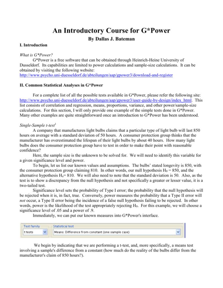
An Introductory Course for G*Power
By Dallas J. Bateman
I. Introduction
What is G*Power?
G*Power is a free software that can be obtained through Heinrich-Heine University of
Dusseldorf. Its capabilities are limited to power calculations and sample-size calculations. It can be
obtained by visiting the following website:
http://www.psycho.uni-duesseldorf.de/abteilungen/aap/gpower3/download-and-register
II. Common Statistical Analyses in G*Power
For a complete list of all the possible tests available in G*Power, please refer the following site:
http://www.psycho.uni-duesseldorf.de/abteilungen/aap/gpower3/user-guide-by-design/index_html. This
list consists of correlation and regression, means, proportions, variance, and other power/sample-size
calculations. For this section, I will only provide one example of the simple tests done in G*Power.
Many other examples are quite straightforward once an introduction to G*Power has been understood.
Single-Sample t-test1
A company that manufactures light bulbs claims that a particular type of light bulb will last 850
hours on average with a standard deviation of 50 hours. A consumer protection group thinks that the
manufacturer has overestimated the lifespan of their light bulbs by about 40 hours. How many light
bulbs does the consumer protection group have to test in order to make their point with reasonable
confidence?
Here, the sample size is the unknown to be solved for. We will need to identify this variable for
a given significance level and power.
To begin, let us list our known values and assumptions. The bulbs’ stated longevity is 850, with
the consumer protection group claiming 810. In other words, our null hypothesis H0 = 850, and the
alternative hypothesis Ha= 810. We will also need to note that the standard deviation is 50. Also, as the
test is to show a discrepancy from the null hypothesis and not specifically a greater or lesser value, it is a
two-tailed test.
Significance level sets the probability of Type I error; the probability that the null hypothesis will
be rejected when it is, in fact, true. Conversely, power measures the probability that a Type II error will
not occur, a Type II error being the incidence of a false null hypothesis failing to be rejected. In other
words, power is the likelihood of the test appropriately rejecting H0. For this example, we will choose a
significance level of .05 and a power of .9.
Immediately, we can put our known measures into G*Power's interface.
We begin by indicating that we are performing a t-test, and, more specifically, a means test
involving a sample's difference from a constant (how much do the reality of the bulbs differ from the
manufacturer's claim of 850 hours?).
The type of power analysis being performed is noted to be an 'A Priori' analysis, a determination
of sample size. From there, we can input the number of tails, the value of our chosen significance level
(α), and the power; 2, .05, and .9, respectively. The only input still requested is the effect size, or the
difference of the null and hypothetical means divided by the standard deviation.
By clicking on the 'Determine' button to the left of
the Effect size input, a new set of input cells is called up, for
the null hypothesis mean (here represented as Mean H0), the
alternative mean (Mean H1), and the standard deviation (SD
σ). As these numbers are known to us (850, 810, and 50),
simply type them in and click 'Calculate and transfer to main
window'. As a result, the effect level's value (given as .8) is
handily computed and inputted.
By pressing the 'Calculate' button in the main window, the desired sample size, among other
statistics, will be produced. These are, in descending order, the Noncentrality parameter δ, the Critical t
(the number of standard deviations from the null mean where an observation becomes statistically
significant), the number of degrees freedom, and the test's actual power. In addition, a graphical
representation of the test is shown, with the sampling distribution a dotted blue line, the population
distribution represented by a solid red line, a red shaded area delineating the probability of a type 1
error, a blue area the type 2 error, and a pair of green lines evocating the critical points t.
To at last answer our question, the sample size is shown to be 19. Thus, no fewer than nineteen
light bulbs must be tested in order to generate a statistically significant result (suggesting a rejection of
the null hypothesis, the manufacturer's claim) with a power of .9.
It is common to want to find the reverse of what was performed above. Supposing only 10 light
bulbs were available for testing, what power would the test have, all else held constant?
The frame of the question is altered by setting the type of power analysis from the 'A Priori'
search for sample size to a 'Post hoc' pursuit of achieved power. Immediately, the input parameters
readjust to replace the power input with one for sample size. As all other variables remain as previous,
the new measure of sample size, 10, is entered in.
Making use of the Calculate button, we receive the new output parameters. This includes the
same statistics as output as with the sample size calculation, only the sample size has been changed to
the power received from the model.
III. Working with Graphics in G*Power
G*Power is a very limited software. It is only used to provide sample-size calculations and
power calculations. The graphs provided are only based on the input parameters required for the
specific tests. Outside of those, there is nothing that a user can do to adjust the visual output of a plot.
Notes
1. The example used here was taken and altered from an online example found at
http://www.ats.ucla.edu/stat/gpower/one_sample.htm (accessed 4/15/2010). To see more
examples using G*Power such as a paired-sample t-test, independent-sample t-test, one-way
ANOVA, or multiple regression, visit http://www.ats.ucla.edu/stat/dae/.