Proceedings of the Twenty-Sixth AAAI Conference on Artificial Intelligence
Matching State-Based Sequences with Rich Temporal Aspects
Aihua Zheng1,2 *Jixin Ma2 Jin Tang1
Bin Luo1
Anhui University, Hefei 230039, China, (00)86 0551 5108445
1
University of Greenwich, London SE10 9LS, United Kingdom, (00)44 020 8331 8539
ahzheng214@gmail.com; j.ma@gre.ac.uk; ahhftang@gmail.com; luobin@ahu.edu.cn
2
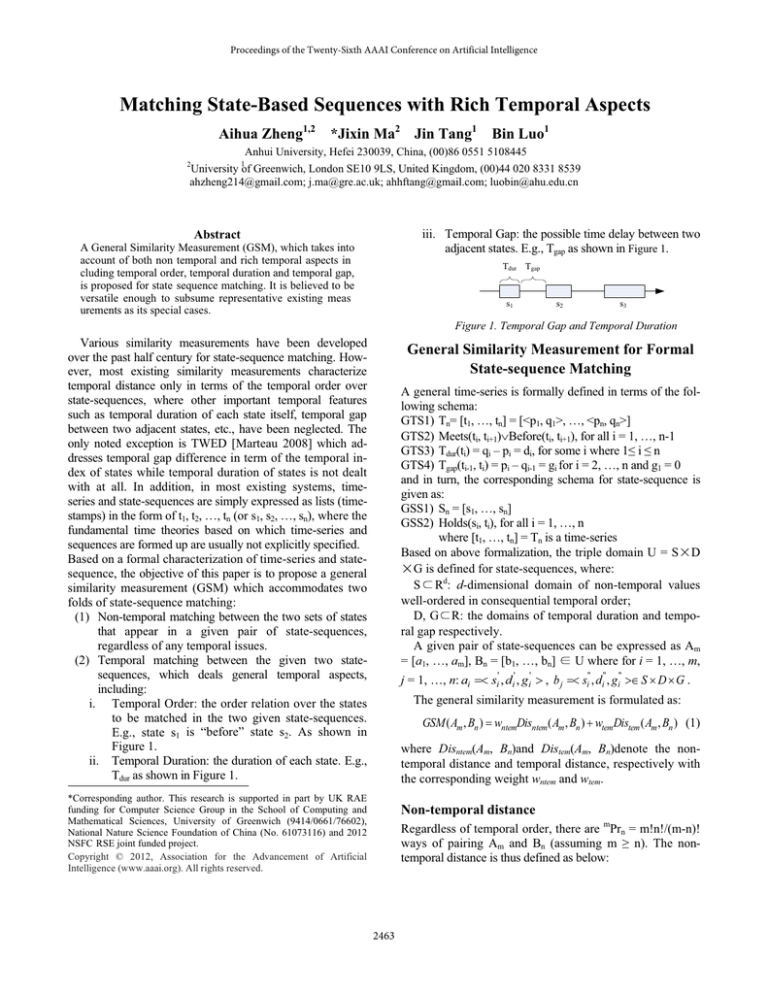
iii. Temporal Gap: the possible time delay between two
adjacent states. E.g., Tgap as shown in Figure 1.
Abstract
A General Similarity Measurement (GSM), which takes into
account of both non temporal and rich temporal aspects in
cluding temporal order, temporal duration and temporal gap,
is proposed for state sequence matching. It is believed to be
versatile enough to subsume representative existing meas
urements as its special cases.
Tdur Tgap
s1
s2
s3
Figure 1. Temporal Gap and Temporal Duration
Various similarity measurements have been developed
over the past half century for state-sequence matching. However, most existing similarity measurements characterize
temporal distance only in terms of the temporal order over
state-sequences, where other important temporal features
such as temporal duration of each state itself, temporal gap
between two adjacent states, etc., have been neglected. The
only noted exception is TWED [Marteau 2008] which addresses temporal gap difference in term of the temporal index of states while temporal duration of states is not dealt
with at all. In addition, in most existing systems, timeseries and state-sequences are simply expressed as lists (timestamps) in the form of t1, t2, …, tn (or s1, s2, …, sn), where the
fundamental time theories based on which time-series and
sequences are formed up are usually not explicitly specified.
Based on a formal characterization of time-series and statesequence, the objective of this paper is to propose a general
similarity measurement (GSM) which accommodates two
folds of state-sequence matching:
(1) Non-temporal matching between the two sets of states
that appear in a given pair of state-sequences,
regardless of any temporal issues.
(2) Temporal matching between the given two statesequences, which deals general temporal aspects,
including:
i. Temporal Order: the order relation over the states
to be matched in the two given state-sequences.
E.g., state s1 is “before” state s2. As shown in
Figure 1.
ii. Temporal Duration: the duration of each state. E.g.,
Tdur as shown in Figure 1.
General Similarity Measurement for Formal
State-sequence Matching
A general time-series is formally defined in terms of the following schema:
GTS1) Tn= [t1, …, tn] = [<p1, q1>, …, <pn, qn>]
GTS2) Meets(ti, ti+1)›Before(ti, ti+1), for all i = 1, …, n-1
GTS3) Tdur(ti) = qi – pi = di, for some i where 1≤ i ≤ n
GTS4) Tgap(ti-1, ti) = pi – qi-1 = gi for i = 2, …, n and g1 = 0
and in turn, the corresponding schema for state-sequence is
given as:
GSS1) Sn = [s1, …, sn]
GSS2) Holds(si, ti), for all i = 1, …, n
where [t1, …, tn] = Tn is a time-series
Based on above formalization, the triple domain U = S D
G is defined for state-sequences, where:
S Rd: d-dimensional domain of non-temporal values
well-ordered in consequential temporal order;
D, G R: the domains of temporal duration and temporal gap respectively.
A given pair of state-sequences can be expressed as Am
= [a1, …, am], Bn = [b1, …, bn]
U where for i = 1, …, m,
'
'
'
j = 1, …, n: ai si , di , gi ! , b j si" , di" , gi" ! S u D u G .
The general similarity measurement is formulated as:
GSM ( Am , Bn ) wntemDisntem ( Am , Bn ) wtem Distem ( Am , Bn ) (1)
where Disntem(Am, Bn)and Distem(Am, Bn)denote the nontemporal distance and temporal distance, respectively with
the corresponding weight wntem and wtem.
*Corresponding author. This research is supported in part by UK RAE
funding for Computer Science Group in the School of Computing and
Mathematical Sciences, University of Greenwich (9414/0661/76602),
National Nature Science Foundation of China (No. 61073116) and 2012
NSFC RSE joint funded project.
Copyright © 2012, Association for the Advancement of Artificial
Intelligence (www.aaai.org). All rights reserved.
Non-temporal distance
Regardless of temporal order, there are mPrn = m!n!/(m-n)!
ways of pairing Am and Bn (assuming m ≥ n). The nontemporal distance is thus defined as below:
2463
Disntem(Am, Bn) = minpr
Prdisntem(pr,
Bn)
Dataset AT&T
face
Method
65.39
OED
76.92
EDR
74.57
LCSS
60.23
CLCS
75.84
ACS
T-WLCS 72.59
GSM
78.36
(2)
Where pr = [pr1,…, prn] and
¦
n
disntem ( pr , Bn )
j 1
wipr disLp ( pr j , s 'j' ) 2 /
¦
n
w
i 1 ipr
Temporal distance
The temporal distance between two given state-sequences
Am and Bn with respect to the 3 temporal aspects is recursively defined as below:
­Distem ( Am1 , Bn ) WdelC (am o I )
°
(3)
Distem ( Am , Bn ) min®Distem ( Am , Bn1 ) WinsC (I o bn )
°Dis ( A , B ) W C (a o b )
sub
m
n
¯ tem m1 n1
where C (a m o I ) , C (I o bn ) and C (am o bn ) denote
the cost function for edit operations deletion, insertion and
substitution, respectively with m, n 1.
­
°
° wi ˜ Ci ( x o y ) if Ci ( x o y ) d G
(4)
C ( x o y) ® i
° k
else
°
¯
Where ( x o y) {(am o I ), (I o bn ), (am o bn )} and k is
a constant usually set either as 0 (to filter out the noise), or
as the current maximum cost (to release the influence of
the noise).
The initialization is set as below:
Distem(A0, B0) = 0,
Distem(A0, Bj) = , for j 1
(5)
Distem(Ai, B0) = , for i 1
The cost functions of GSM are defined as below:
­
distLp (0, s"j ) if si' I
°
°
(7)
CTord (ai o b j ) ®distLp ( si' ,0) if s"j I
°dist ( s ' , s" ) else
Lp i
j
°
¯
Table 1. Clustering accuracy comparison
Table 2 below shows the average mean and standard deviation (STD) of retrieval precision on each noised dataset
with Gaussian noise with respect to different means and
variances which verifies the effectiveness of GSM.
Dataset
Statistic
Mean
ERP
STD
Mean
DTW
STD
Mean
TWED
STD
¦
CTdur (ai o b j )
CTgap(ai o b j )
­
dist Lp (0, d "j ) if d i' I
°
°
'
"
®dist Lp (d i ,0) if d j I
°dist (d ' , d " ) else
Lp i
j
°
¯
­
distLp (0, g "j ) if g i' I
°
°
'
"
®distLp ( g i ,0) if g j I
°dist ( g ' , g " ) else
Lp
i
j
°
¯
Bin
USPS MNIST COIL20 Isolet1 Alpha
60.50 54.95
59.84 65.85 68.96
66.87 66.31
61.28 70.49 71.32
66.25 52.96
53.74
60.37 56.44
57.64 50.35
51.87
55.24 53.49
73.85 55.66
60.55
64.85 60.55
70.17 58.23
66.62
66.36 61.21
76.41 66.35
69.20 75.58 72.66
GSM
AT&T USPS MNIST COIL20 Isolet1 Bin
face
Alpha
63.71
0.1249
73.37
0.1932
79.95
0.0993
65.60
0.1391
72.29
0.1128
75.30
0.1025
Mean 85.65 80.54
59.48 61.53 74.66 71.25
0.1742 0.2519 0.1285 0.1595
65.79 73.11 78.51 74.29
0.1890 0.1438 0.0891 0.1032
68.80 72.96 79.38 76.90
0.1359 0.1235 0.0940 0.0895
74.82
78.44
84.19 82.84
STD 0.0632 0.0738 0.1022 0.0983 0.0593 0.738
Table 2. Statistic of the retrieval precision of noised dataset
Table 3 presents the classification precision with different combinations of temporal aspects. It shows that GSM is
capable of tackling most matching tasks involving timeseries and state-sequence data, especially with different
temporal matching requirements.
Dataset AT&T USPS MNIST COIL20 Isolet1 Binary
face
Alpha
Aspects
Tord
87.50 90.69 85.40 87.08 89.23 86.00
Tdur
91.00 86.56 82.20 88.75 90.13 87.18
(8)
(9)
Tgap
88.50
87.12
83.80
88.47
89.87 87.77
Tord+Tdur
89.50
89.61
86.80
89.86
92.69 90.73
Tord +Tgap
90.50
91.44
89.20
89.72
93.21 89.15
Tdur + Tgap
87.50
90.77
86.60
89.86
92.82 90.34
Tord+Tgap+Tdur
94.00
93.53
89.80
91.81
94.23 92.90
Table 3. Classification precision with various combinations
Experimental Results
Reference
The GSM has been tested on 6 benchmark datasets. Table
1 shows the clustering accuracy of K-means on each of
these dataset. Generally speaking, GSM has the highest accuracy which means it outperforms all the other Binaryvalue Measurements.
Marteau P.F. “Time Warp Edit Distances with Stiffness
Adjustment for Time Series Matching”. IEEE Trans. on
Pattern Analysis and Machine Intelligence, In Press(0):115, April 2008.
2464