Proceedings of the Fifth Annual Symposium on Combinatorial Search
Fast Path Planning through Segmentation of the
Map into Manhattan-Cohesive Areas
Ioannis Papikas and Ioannis Refanidis
Department of Applied Informatics
University of Macedonia, Thessaloniki, Greece
mai124@uom.gr and yrefanid@uom.gr
Abstract
This paper presents a method for fast planning within
arbitrary maps, through segmentation of the map into
Manhattan-cohesive areas. A Manhattan-cohesive area
is a connected part of the map where the optimal distance between any two points in the area is equal to their
Manhattan distance. We adopt a four directions Manhattan distance, where diagonal moves are allowed. In the
paper we present the method we adopted to fragmentize
the map, as well the method to extract the paths. The
proposed method produces nearly optimal plans quite
efficiently.
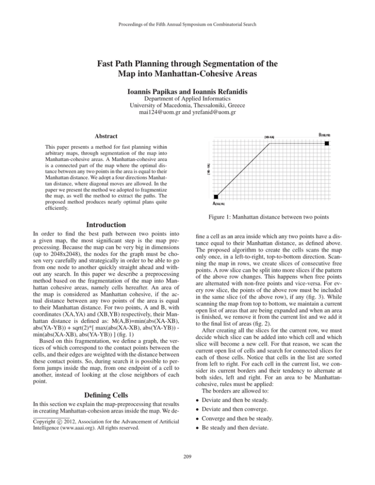
Figure 1: Manhattan distance between two points
Introduction
In order to find the best path between two points into
a given map, the most significant step is the map preprocessing. Because the map can be very big in dimensions
(up to 2048x2048), the nodes for the graph must be chosen very carefully and strategically in order to be able to go
from one node to another quickly straight ahead and without any search. In this paper we describe a preprocessing
method based on the fragmentation of the map into Manhattan cohesive areas, namely cells hereafter. An area of
the map is considered as Manhattan cohesive, if the actual distance between any two points of the area is equal
to their Manhattan distance. For two points, A and B, with
coordinates (XA,YA) and (XB,YB) respectively, their Manhattan distance is defined as: M(A,B)=min(abs(XA-XB),
abs(YA-YB)) + sqrt(2)*[ max(abs(XA-XB), abs(YA-YB)) min(abs(XA-XB), abs(YA-YB)) ] (fig. 1)
Based on this fragmentation, we define a graph, the vertices of which correspond to the contact points between the
cells, and their edges are weighted with the distance between
these contact points. So, during search it is possible to perform jumps inside the map, from one endpoint of a cell to
another, instead of looking at the close neighbors of each
point.
fine a cell as an area inside which any two points have a distance equal to their Manhattan distance, as defined above.
The proposed algorithm to create the cells scans the map
only once, in a left-to-right, top-to-bottom direction. Scanning the map in rows, we create slices of consecutive free
points. A row slice can be split into more slices if the pattern
of the above row changes. This happens when free points
are alternated with non-free points and vice-versa. For every row slice, the points of the above row must be included
in the same slice (of the above row), if any (fig. 3). While
scanning the map from top to bottom, we maintain a current
open list of areas that are being expanded and when an area
is finished, we remove it from the current list and we add it
to the final list of areas (fig. 2).
After creating all the slices for the current row, we must
decide which slice can be added into which cell and which
slice will become a new cell. For that reason, we scan the
current open list of cells and search for connected slices for
each of those cells. Notice that cells in the list are sorted
from left to right. For each cell in the current list, we consider its current borders and their tendency to alternate at
both sides, left and right. For an area to be Manhattancohesive, rules must be applied:
The borders are allowed to:
Defining Cells
• Deviate and then be steady.
In this section we explain the map-preprocessing that results
in creating Manhattan-cohesion areas inside the map. We de-
• Deviate and then converge.
• Converge and then be steady.
c 2012, Association for the Advancement of Artificial
Copyright Intelligence (www.aaai.org). All rights reserved.
• Be steady and then deviate.
209
Figure 2: Creating cells on map-segment
Figure 4: Graph created
we retain the two areas being connected. With that information, we know which cells are neighbors and which are not
(fig. 4).
Concerning the edges of the graph, we create an edge for
each pair of nodes that involve the same cell. The weights
of these edges are equal to the Manhattan distance of these
nodes, which, according to our assumption for cell creation, is their actual distance. The computation of the edges’
weights is performed at the time of cell formation.
Figure 3: Slice pattern
Searching for the Path
For a specific path-planning problem, we introduce two additional nodes in the graph, corresponding to the start and
goal point respectively. These nodes are connected with
edges with all nodes that involve their cells. Before the actual search, we check two more things:
The borders cannot converge and then deviate. So, when
its the time to choose which slices can be inserted in which
cells, we take into consideration the above restrictions. For
each cell, many slices may be candidates to be inserted. We
choose the slice with the biggest width and only if its more
than 10% of the last width of the cell (last width is the width
of the last slice that inserted in that cell). Slices that are not
inserted in existing areas, initiate new cells.
Each cell is stored as a structure consisting of the row
where it starts, the total number of rows it spans and for each
row in between, two vectors where we keep the start and the
end position of each slice. This is a compact way of storing
every cell, instead of storing each point of the map, and is
much easier and faster to see if a point is within an area.
Finally, we have to define the points of connection between any two adjacent cells. Two adjacent cells can be connected vertically or horizontally. Vertically, when between
two or more candidate slices the cell chooses one of them,
the rest will become a new cell or will be inserted into another area. Horizontally, when two slices in the same row
are connected (being separated because of the previous row
pattern) but are inserted into different cells.
• Whether the points are in the same cell.
• Whether the points, although not in the same cell, can be
connected with a Manhattan path.
In both of the above occasions, we connect the two points
and there is no search at all. If none of the above is true,
search starts. And now it is only matter of time and cpu cycles to find a nearly optimal path among the nodes we have
created. As for a search algorithm, we adopted A* coupled
with Manhattan distance as its heuristic.
Conclusions and Future Work
Our method finds nearly optimal paths. The loss of optimality is due to the selection of contact points at the contact
area of adjacent cells. So, we are working on improving the
strategy for selecting the contact points and, consequently
the nodes of the graph. The decision will be based on the
relative position of the cells, the size and the position of the
other nodes-neighbors.
Another improvement is the way the path is being extracted. During backtracking and path extraction, we can
check if a node can be connected directly with its grandparent, i.e., bypassing its parent, and continue up the tree
until there is no connection possible. That way, we may slow
down the algorithm but we may be able to extract a shorter
path.
Creating the Graph
Having found the cells and the connection points, we proceed with creating a graph. A node of this graph consists of
a pair of adjacent points, one from each adjacent cell, connecting them either vertically or horizontally. Horizontally,
the node is usually only one point of connection, so we create a node with the two points being side by side. Vertically,
there are usually multiple pairs of adjacent points that form
the connection area. We choose the two pairs of points on
the right and on the left side of the connection area, and if
the width of the connection area is bigger than 10 points, we
take another node in the middle of this area. At each node,
210